
Overview
In this article, we demonstrate how to train a TensorFlow model using the CIFAR-10 dataset, quantize the model, and use it for inference on a Raspberry Pi 3.
As the use of image recognition expands, the number of use cases requiring real-time recognition processing by edge devices is increasing.
NEXTY Electronics handles a variety of edge devices related to image recognition and AI and is working on image recognition and AI-related initiatives. As a sample of one of these initiatives, we will now introduce a series of processes that utilize Google Colaboratory to carry out everything from model training to quantization, ultimately achieving efficient inference on a Raspberry Pi 3.
Google Colaboratory environment settings
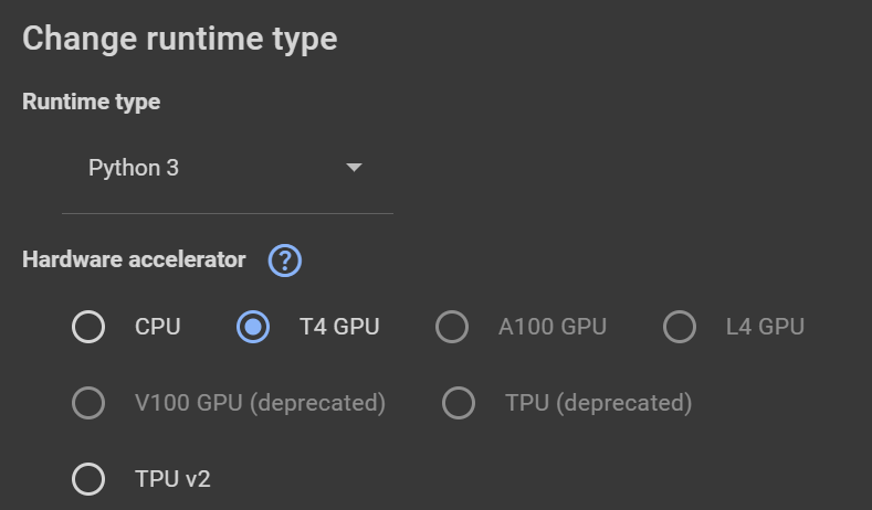
I selected RuntimeChange runtime type from the menu and selected T4 GPU.
Mounting Google Drive and installing the library
First, mount your Google Drive and install the required libraries.
(The first time you run it, a window will appear asking you to connect to Google Drive. Please log in with your Google account and then connect.)
| from google.colab import drive rive.mount('/content/gdrive') !pip install tensorflow==2.15.0 |
|---|
Importing required libraries
Next, import the required libraries:
| import matplotlib.pyplot as plt import numpy as np import time import datetime from sklearn.metrics import accuracy_score, precision_score, recall_score, f1_score import keras from keras.datasets import cifar10 from keras.applications import VGG16 from keras.layers import Dense, Flatten from keras.models import Model from keras.utils import to_categorical from keras.optimizers import Adam import tensorflow as tf from tensorflow.keras import Input from tensorflow.keras.layers import Conv2D, MaxPooling2D, Flatten, Dense |
|---|
Check the version of each module
| print(f"Keras version: {keras.__version__}") print(f"TensorFlow version: {tf.__version__}") print(f"scikit-learn version: {sklearn.__version__}") print(f"matplotlib version: {matplotlib.__version__}") print(f"NumPy version: {np.__version__}") |
|---|
- Keras version: 2.15.0
- TensorFlow version: 2.15.0
- scikit-learn version: 1.2.2
- matplotlib version: 3.7.1
- NumPy version: 1.25.2
Loading and preprocessing the CIFAR-10 dataset
Load the CIFAR-10 dataset and perform preprocessing.
| # Load CIFAR10 data (train_images, train_labels), (test_images, test_labels) = cifar10.load_data() # Convert class vectors to binary class matrices. train_labels = to_categorical(train_labels, 10) test_labels = to_categorical(test_labels, 10) # Normalize pixel values to be between 0 and 1 train_images, test_images = train_images / 255.0, test_images / 255.0 |
|---|
Model selection and construction
Choose whether to use VGG16 or a custom model.
In this example, we use the pre-built VGG16 model.
| use_vgg16 = True # This is the flag. If it is True, VGG16 is used. Otherwise, Your custom model is used. model_name = "" # Get the current date and time now = datetime.datetime.now() if use_vgg16: # VGG16 Model model_name = "vgg_16" + now.strftime("%Y%m%d_%H%M%S") baseModel = VGG16(weights="imagenet", include_top=False, input_shape=(32,32, 3)) headModel = baseModel.output headModel = Flatten(name="flatten")(headModel) headModel = Dense(512, activation="relu")(headModel) headModel = Dense(10, activation="softmax")(headModel) model = Model(inputs=baseModel.input, outputs=headModel) model.compile(optimizer=Adam(), loss='categorical_crossentropy', metrics= ['accuracy']) else: # Custom Model model_name = "custom_model" + now.strftime("%Y%m%d_%H%M%S") input_tensor = Input(shape=(32, 32, 3)) # Here you can manually change the number of layers, filters, kernel sizes etc. x = Conv2D(64, (3, 3), padding='same', activation='relu')(input_tensor) x = Conv2D(64, (3, 3), padding='same', activation='relu')(x) x = MaxPooling2D((2, 2))(x) x = Conv2D(128, (3, 3), padding='same', activation='relu')(x) x = Conv2D(128, (3, 3), padding='same', activation='relu')(x) x = MaxPooling2D((2, 2))(x) x = Conv2D(256, (3, 3), padding='same', activation='relu')(x) x = Conv2D(256, (3, 3), padding='same', activation='relu')(x) x = MaxPooling2D((2, 2))(x) x = Flatten(name="flatten")(x) x = Dense(512, activation="relu")(x) output_tensor = Dense(10, activation="softmax")(x) # Create the model model = Model(inputs=input_tensor, outputs=output_tensor) model.summary() |
|---|
| _________________________________________________________________ Layer (type) Output Shape Param # ================================================================= input_3 (InputLayer) [(None, 32, 32, 3)] 0 block1_conv1 (Conv2D) (None, 32, 32, 64) 1792 block1_conv2 (Conv2D) (None, 32, 32, 64) 36928 block1_pool (MaxPooling2D) (None, 16, 16, 64) 0 block2_conv1 (Conv2D) (None, 16, 16, 128) 73856 block2_conv2 (Conv2D) (None, 16, 16, 128) 147584 block2_pool (MaxPooling2D) (None, 8, 8, 128) 0 block3_conv1 (Conv2D) (None, 8, 8, 256) 295168 block3_conv2 (Conv2D) (None, 8, 8, 256) 590080 block3_conv3 (Conv2D) (None, 8, 8, 256) 590080 block3_pool (MaxPooling2D) (None, 4, 4, 256) 0 block4_conv1 (Conv2D) (None, 4, 4, 512) 1180160 block4_conv2 (Conv2D) (None, 4, 4, 512) 2359808 block4_conv3 (Conv2D) (None, 4, 4, 512) 2359808 block4_pool (MaxPooling2D) (None, 2, 2, 512) 0 block5_conv1 (Conv2D) (None, 2, 2, 512) 2359808 block5_conv2 (Conv2D) (None, 2, 2, 512) 2359808 block5_conv3 (Conv2D) (None, 2, 2, 512) 2359808 block5_pool (MaxPooling2D) (None, 1, 1, 512) 0 flatten (Flatten) (None, 512) 0 dense_4 (Dense) (None, 512) 262656 dense_5 (Dense) (None, 10) 5130 ================================================================= Total params: 14982474 (57.15 MB) Trainable params: 14982474 (57.15 MB) Non-trainable params: 0 (0.00 Byte) _________________________________________________________________ |
|---|
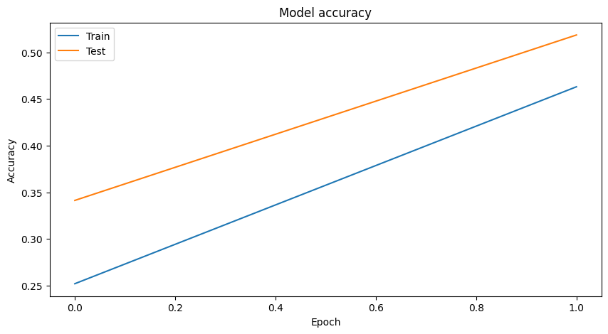
Model training: Experiment for 2 epochs
Compile and train the model.
First, set Epoch to 2 and try learning under conditions that are not expected to produce very high accuracy.
| # Training epochs=2 model.compile(optimizer=Adam(), loss='categorical_crossentropy', metrics= ['accuracy']) history = model.fit(train_images, train_labels, batch_size=64, epochs=epochs, validation_data=(test_images, test_labels)) |
|---|
- Learning log excerpt
| Epoch 1/2 782/782 [==============================]- 42s 41ms/step - loss: 1.8300 - accuracy: 0.2521 - val_loss: 1.6348 - val_accuracy: 0.3413 Epoch 2/2 782/782 [==============================] - 29s 38ms/step - loss: 1.3756 - accuracy: 0.4630 - val_loss: 1.3297 - val_accuracy: 0.5185 |
|---|
Visualizing training results
| # Visualize Training Graph # Plotting the accuracy plt.figure(figsize=(10,5)) plt.plot(history.history['accuracy']) plt.plot(history.history['val_accuracy']) plt.title('Model accuracy') plt.ylabel('Accuracy') plt.xlabel('Epoch') plt.legend(['Train', 'Test'], loc='upper left') plt.show() # Plotting the loss plt.figure(figsize=(10,5)) plt.plot(history.history['loss']) plt.plot(history.history['val_loss']) plt.title('Model loss') plt.ylabel('Loss') plt.xlabel('Epoch') plt.legend(['Train', 'Test'], loc='upper left') plt.show() |
|---|
Model evaluation and prediction
| # Predictions class_names = ['airplane', 'automobile', 'bird', 'cat', 'deer', 'dog', 'frog', 'horse', 'ship', 'truck'] # Start time record start_time = time.time() # Predictions predictions = model.predict(test_images) # End time record end_time = time.time() # Convert predictions and test labels to 1D arrays test_predictions = np.argmax(predictions, axis=1) # <-- Here we should use 'predictions' test_labels_1d = np.argmax(test_labels, axis=1) # Calculate accuracy accuracy = accuracy_score(test_labels_1d, test_predictions) # Calculate precision precision = precision_score(test_labels_1d, test_predictions, average='weighted') # Calculate recall recall = recall_score(test_labels_1d, test_predictions, average='weighted') # Calculate F1 score f1 = f1_score(test_labels_1d, test_predictions, average='weighted') # Count the number of correct predictions correct_predictions = np.sum(np.argmax(test_labels, axis=1) == np.argmax(predictions, axis=1)) # Calculate total inference time total_inference_time = end_time - start_time # Calculate inference time per image inference_time_per_image = total_inference_time / test_images.shape[0] # Calculate frames per second (fps) fps = 1 / inference_time_per_image # Calculate accuracy test_accuracy = correct_predictions / test_images.shape[0] # Get the number of model parameters num_params = model.count_params() print("\033[92m") print("---Tensorflow") print(f"Total inference time: {total_inference_time:.2f} seconds") print(f"Inference time per image: {inference_time_per_image:.6f} seconds") print(f"Inference speed: {fps:.2f} frames per second") print(f"Test accuracy: {test_accuracy * 100:.2f}%") print(f"Correct predictions: {correct_predictions}/{test_images.shape[0]}") print(f"Accuracy: {accuracy}") print(f"Precision: {precision}") print(f"Recall: {recall}") print(f"F1 Score: {f1}") print(f"Number of parameters: {num_params}") print(f"\033[0m") |
|---|
- Total inference time: 3.62 seconds
- Inference time per image: 0.000362 seconds
- Inference speed: 2762.24 frames per second
- Test accuracy: 51.85%
- Correct predictions: 5185/10000
- Accuracy: 0.5185
- Precision: 0.5460565026512546
- Recall: 0.5185
- F1 Score: 0.5121520088704362
- Number of parameters: 14982474
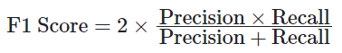
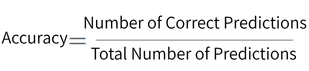
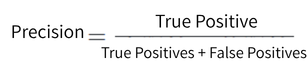
Model evaluation metrics: English version
The following formula shows how the evaluation index is calculated:
- Accuracy
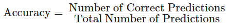
- Precision
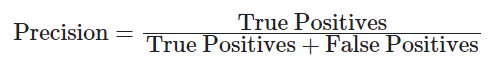
- Recall rate
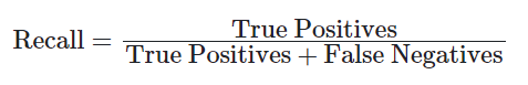
- F1 Score
Model evaluation index: Japanese version
The following formula shows how the evaluation index is calculated:
- Accuracy
- Precision
- Recall rate
- F1 Score
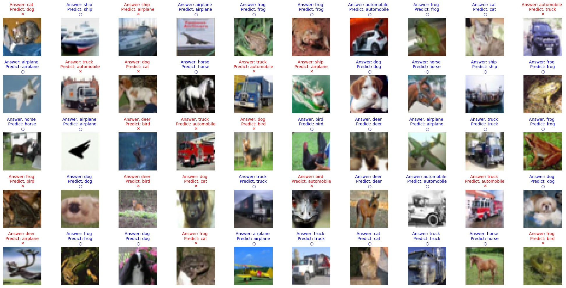
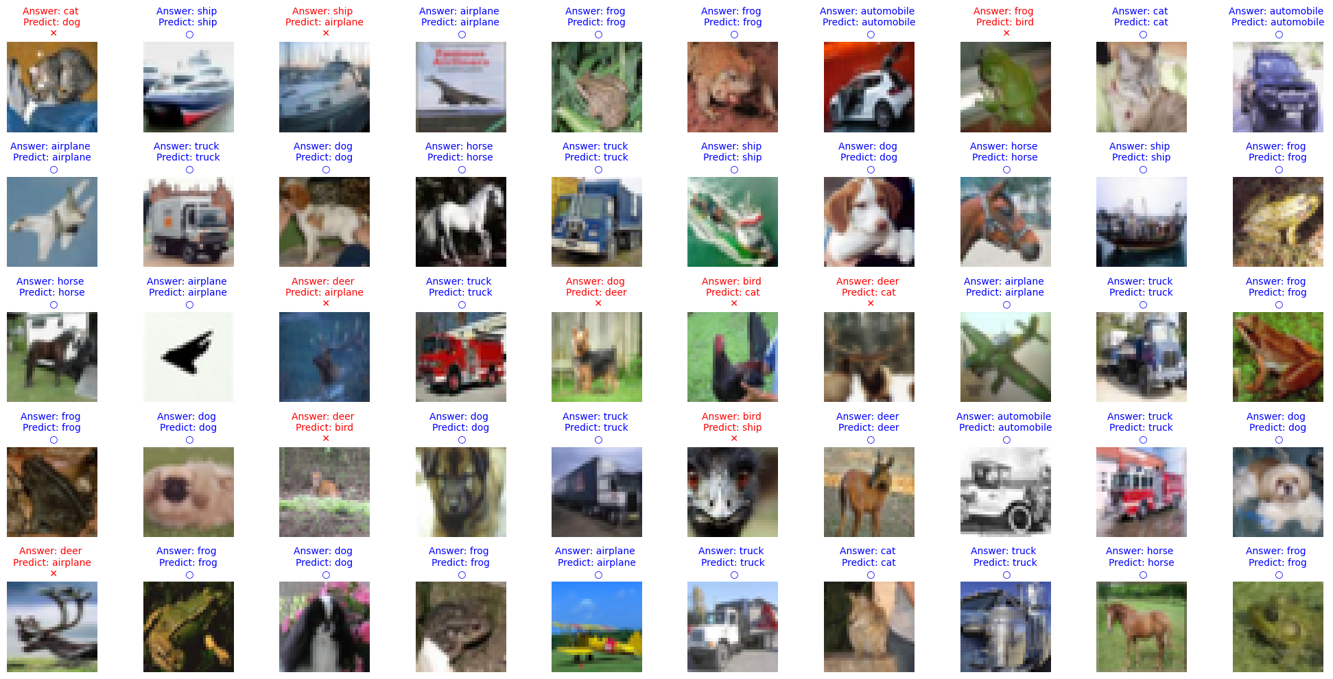
Visualization of prediction results
The number of correct answers is 5185/10000 as shown above, but let's check it in image format.
It displays random images from the test data and compares the predictions with the correct answer.
| num_rows = 5 num_cols = 10 num_images = num_rows*num_cols fig, axes = plt.subplots(num_rows, num_cols, figsize=(20, 2 * num_rows)) # Adjust the figure size axes = axes.ravel() for i in np.arange(0, num_images): axes[i].imshow(test_images[i]) if np.argmax(test_labels[i]) == np.argmax(predictions[i]): axes[i].set_title("Answer: %s \nPredict: %s\n \u25CB" % (class_names[np.argmax(test_labels[i])], class_names[np.argmax(predictions[i])]), fontsize=10, color='blue') else: axes[i].set_title("Answer: %s \nPredict: %s\n \u2715" % (class_names[np.argmax(test_labels[i])], class_names[np.argmax(predictions[i])]), fontsize=10, color='red') axes[i].axis('off') plt.tight_layout() # Apply tight_layout |
|---|
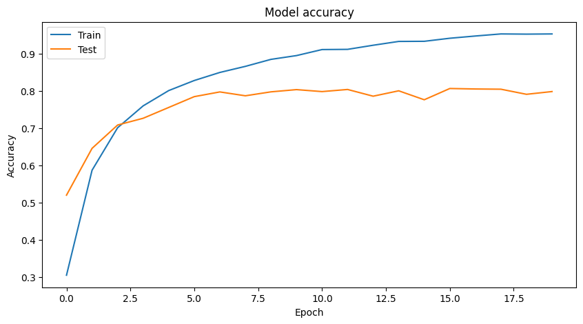
Model training: Experiment for 20 epochs
| # Training epochs=20 model.compile(optimizer=Adam(), loss='categorical_crossentropy', metrics= ['accuracy']) history = model.fit(train_images, train_labels, batch_size=64, epochs=epochs, validation_data=(test_images, test_labels)) |
|---|
- Learning log excerpt
| Epoch 1/20 782/782 [==============================] - 49s 51ms/step - loss: 1.7404 - accuracy: 0.3044 - val_loss: 1.2784 - val_accuracy: 0.5199 Epoch 2/20 782/782 [==============================] - 33s 42ms/step - loss: 1.1353 - accuracy: 0.5870 - val_loss: 1.0319 - val_accuracy: 0.6459 Epoch 3/20 782/782 [==============================] - 34s 44ms/step - loss: 0.8738 - accuracy: 0.7014 - val_loss: 0.8739 - val_accuracy: 0.7087 Epoch 4/20 782/782 [==============================] - 38s 49ms/step - loss: 0.7150 - accuracy: 0.7603 - val_loss: 0.7924 - val_accuracy: 0.7269 Epoch 5/20 782/782 [==============================] - 31s 40ms/step - loss: 0.6050 - accuracy: 0.8014 - val_loss: 0.8037 - val_accuracy: 0.7560 Epoch 6/20 782/782 [==============================] - 31s 40ms/step - loss: 0.5321 - accuracy: 0.8285 - val_loss: 0.6816 - val_accuracy: 0.7851 Epoch 7/20 782/782 [==============================] - 31s 40ms/step - loss: 0.4607 - accuracy: 0.8502 - val_loss: 0.6683 - val_accuracy: 0.7978 Epoch 8/20 782/782 [==============================] - 32s 41ms/step - loss: 0.4130 - accuracy: 0.8666 - val_loss: 0.6847 - val_accuracy: 0.7874 Epoch 9/20 782/782 [==============================] - 32s 41ms/step - loss: 0.3603 - accuracy: 0.8854 - val_loss: 0.6863 - val_accuracy: 0.7980 Epoch 10/20 782/782 [==============================] - 32s 41ms/step - loss: 0.3283 - accuracy: 0.8956 - val_loss: 0.7302 - val_accuracy: 0.8040 Epoch 11/20 782/782 [==============================] - 31s 40ms/step - loss: 0.2775 - accuracy: 0.9118 - val_loss: 0.7026 - val_accuracy: 0.7987 Epoch 12/20 782/782 [==============================] - 31s 40ms/step - loss: 0.2710 - accuracy: 0.9124 - val_loss: 0.7211 - val_accuracy: 0.8044 Epoch 13/20 782/782 [==============================] - 31s 40ms/step - loss: 0.2417 - accuracy: 0.9235 - val_loss: 0.7624 - val_accuracy: 0.7863 Epoch 14/20 782/782 [==============================] - 32s 41ms/step - loss: 0.2163 - accuracy: 0.9337 - val_loss: 0.8034 - val_accuracy: 0.8008 Epoch 15/20 782/782 [==============================] - 31s 40ms/step - loss: 0.2113 - accuracy: 0.9341 - val_loss: 0.8858 - val_accuracy: 0.7767 Epoch 16/20 782/782 [==============================] - 31s 39ms/step - loss: 0.1905 - accuracy: 0.9423 - val_loss: 0.7814 - val_accuracy: 0.8070 Epoch 17/20 782/782 [==============================] - 31s 40ms/step - loss: 0.1669 - accuracy: 0.9483 - val_loss: 0.8559 - val_accuracy: 0.8057 Epoch 18/20 782/782 [==============================] - 31s 40ms/step - loss: 0.1532 - accuracy: 0.9539 - val_loss: 0.8492 - val_accuracy: 0.8051 Epoch 19/20 782/782 [==============================] - 31s 40ms/step - loss: 0.1540 - accuracy: 0.9534 - val_loss: 0.8842 - val_accuracy: 0.7914 Epoch 20/20 782/782 [==============================] - 32s 41ms/step - loss: 0.1515 - accuracy: 0.9539 - val_loss: 0.9053 - val_accuracy: 0.7988 |
|---|
Visualizing training results
Plot the accuracy and loss during the training process.
| # Visualize Training Graph # Plotting the accuracy plt.figure(figsize=(10,5)) plt.plot(history.history['accuracy']) plt.plot(history.history['val_accuracy']) plt.title('Model accuracy') plt.ylabel('Accuracy') plt.xlabel('Epoch') plt.legend(['Train', 'Test'], loc='upper left') plt.show() # Plotting the loss plt.figure(figsize=(10,5)) plt.plot(history.history['loss']) plt.plot(history.history['val_loss']) plt.title('Model loss') plt.ylabel('Loss') plt.xlabel('Epoch') plt.legend(['Train', 'Test'], loc='upper left') plt.show() |
|---|
Model evaluation and prediction
The performance of the model is evaluated using test data and prediction results are output.
| # Predictions class_names = ['airplane', 'automobile', 'bird', 'cat', 'deer', 'dog', 'frog', 'horse', 'ship', 'truck'] # Start time record start_time = time.time() # Predictions predictions = model.predict(test_images) # End time record end_time = time.time() # Convert predictions and test labels to 1D arrays test_predictions = np.argmax(predictions, axis=1) test_labels_1d = np.argmax(test_labels, axis=1) # Calculate accuracy accuracy = accuracy_score(test_labels_1d, test_predictions) # Calculate precision precision = precision_score(test_labels_1d, test_predictions, average='weighted') # Calculate recall recall = recall_score(test_labels_1d, test_predictions, average='weighted') # Calculate F1 score f1 = f1_score(test_labels_1d, test_predictions, average='weighted') # Count the number of correct predictions correct_predictions = np.sum(np.argmax(test_labels, axis=1) == np.argmax(predictions, axis=1)) # Calculate total inference time total_inference_time = end_time - start_time # Calculate inference time per image inference_time_per_image = total_inference_time / test_images.shape[0] # Calculate frames per second (fps) fps = 1 / inference_time_per_image # Calculate accuracy test_accuracy = correct_predictions / test_images.shape[0] # Get the number of model parameters num_params = model.count_params() print("\033[92m") print("---Tensorflow") print(f"Total inference time: {total_inference_time:.2f} seconds") print(f"Inference time per image: {inference_time_per_image:.6f} seconds") print(f"Inference speed: {fps:.2f} frames per second") print(f"Test accuracy: {test_accuracy * 100:.2f}%") print(f"Correct predictions: {correct_predictions}/{test_images.shape[0]}") print(f"Accuracy: {accuracy}") print(f"Precision: {precision}") print(f"Recall: {recall}") print(f"F1 Score: {f1}") print(f"Number of parameters: {num_params}") print("\033[0m") |
|---|
- Total inference time: 3.44 seconds
- Inference time per image: 0.000344 seconds
- Inference speed: 2910.39 frames per second
- Test accuracy: 79.88%
- Correct predictions: 7988/10000
- Accuracy: 0.7988
- Precision: 0.8079718674357317
- Recall: 0.7988
- F1 Score: 0.8000619454577802
- Number of parameters: 14982474
Visualization of prediction results
It displays random images from the test data and compares the predictions with the correct answer.
| num_rows = 5 num_cols = 10 num_images = num_rows*num_cols fig, axes = plt.subplots(num_rows, num_cols, figsize=(20, 2 * num_rows)) # Adjust the figure size axes = axes.ravel() for i in np.arange(0, num_images): axes[i].imshow(test_images[i]) if np.argmax(test_labels[i]) == np.argmax(predictions[i]): axes[i].set_title("Answer: %s \nPredict: %s\n \u25CB" % (class_names[np.argmax(test_labels[i])], class_names[np.argmax(predictions[i])]), fontsize=10, color='blue') else: axes[i].set_title("Answer: %s \nPredict: %s\n \u2715" % (class_names[np.argmax(test_labels[i])], class_names[np.argmax(predictions[i])]), fontsize=10, color='red') axes[i].axis('off') plt.tight_layout() # Apply tight_layout |
|---|
Comparison of Epoch2 and Epoch20
| index | Epoch 2 | Epoch 20 |
|---|---|---|
| Accuracy | 0.5185(51.85%) | 0.7988(79.88%) |
| Precision | 0.5461 | 0.8080 |
| Recall (recall rate) | 0.5185 | 0.7988 |
| F1 Score | 0.5122 | 0.8001 |
- Accuracy
The accuracy for Epoch 2 was 51.85%, which indicates that the model is not predicting randomly, but is almost half accurate.
In Epoch 20, the accuracy improved to 79.88%, indicating that the model is now able to classify more accurately.
- Precision
Precision indicates the percentage of correctly classified positive examples.
In Epoch 2, it was 0.5461, but in Epoch 20 it improved to 0.8080.
This indicates that the model is now able to predict positive examples more accurately.
- Recall
Recall indicates the proportion of correctly classified positive examples.
In Epoch 2, it was 0.5185, but in Epoch 20, it improved to 0.7988.
This indicates that the model is now able to predict many positive examples without missing any.
- F1 Score
The F1 score is the harmonic mean of Precision and Recall, and is a balanced evaluation metric.
In Epoch 2, it was 0.5122, but in Epoch 20, it improved to 0.8001.
This indicates that the model has a more balanced performance overall.
- comprehensive evaluation
Comparing Epoch2 and Epoch20, we can see that the Epoch20 model is clearly superior. As training continues, the model's accuracy, inference speed, precision, recall, and F1 score all improve.
This is likely due to the model learning more data and optimizing its parameters.
- OTHERS supplementary information
- Model training process
In the early epochs, the model is still in the process of finding the optimal weights, so accuracy and other metrics tend to be low. By increasing the number of epochs, the model will learn the features of the data better, adjust the parameters, and improve performance.
- Overfitting concerns
As the number of epochs increases, the risk of overfitting to the training data increases. Currently, the results of epoch 20 show no signs of overfitting, but evaluation on the validation dataset is important for continued training.
- Hyperparameter Tuning
Tuning hyperparameters such as learning rate and batch size can affect model performance, so finding the right hyperparameters is important.
Overall, we can see that increasing the number of epochs significantly improves the accuracy of the model, indicating that the learning process is progressing smoothly.
Saving a Keras model
This block saves a trained Keras model in HDF5 format (.h5).
Use the model_name variable to define the full path of the model file and use model.save to save the model.
| full_model_name_h5 = "/content/gdrive/MyDrive/Colab Notebooks/{}.h5".format(model_name) model.save(full_model_name_h5) |
|---|
Converting the model to TensorFlow Lite
This block converts a saved Keras model to the TensorFlow Lite format.
First, load the model using tf.keras.models.load_model.
Next, create a TFLiteConverter object and configure it to convert the model using quantization (converter.optimizations = [tf.lite.Optimize.DEFAULT]).
Finally, we convert the model and store the converted data in the tflite_model variable.
| import tensorflow as tf # Load the model model = tf.keras.models.load_model(full_model_name_h5) # Convert the model to the TensorFlow Lite format with quantization converter = tf.lite.TFLiteConverter.from_keras_model(model) # Convert float32 to int8 converter.optimizations = [tf.lite.Optimize.DEFAULT] tflite_model = converter.convert() # Save the model to disk full_model_name_tflite = "/content/gdrive/MyDrive/Colab Notebooks/{}.tflite".format(model_name) open(full_model_name_tflite, "wb").write(tflite_model) |
|---|
Loading and running inference on a TensorFlow Lite model
Load the converted TensorFlow Lite model and run inference on a single test image.
1.Create a TFLiteInterpreter object, specify the model path, and allocate memory for the tensors.
2. Next, we get the details of the input and output tensors. We prepare the input data by reshaping the test image and converting it to float32 format.
3. Set the input tensor to point to the prepared data and use interpreter.invoke to run inference.
4. Finally, take the output data and get the predicted class based on the maximum value of the output.
| # Load TFLite model and allocate tensors interpreter = tf.lite.Interpreter(model_path=full_model_name_tflite) interpreter.allocate_tensors() # Get input and output tensors input_details = interpreter.get_input_details() output_details = interpreter.get_output_details() # Prepare the input data input_shape = input_details[0]['shape'] input_data = np.expand_dims(test_images[i], axis=0).astype("float32") # Assuming you are checking for `i`th image # Set the tensor to point to the input data to be inferred interpreter.set_tensor(input_details[0]['index'], input_data) # Run the inference interpreter.invoke() # Get the output from the inference output_data = interpreter.get_tensor(output_details[0]['index']) # Get the output class output_class = np.argmax(output_data) |
|---|
Performance evaluation of TensorFlow Lite models
We evaluate the performance of the TensorFlow Lite model on the entire test dataset.
1. Import the libraries required to calculate the evaluation metrics. Prepare the input data by getting the input shape from the model.
2. Create a list, predictions, to store the predictions for all test images. Start recording the time and iterate over all test images.
3. In a loop, prepare the input data for each image, set the input tensor, run inference, get the output, and add the prediction to the predictions list.
4. After iterating through all the images, record the time. Convert the predictions and test labels into 1D arrays for easier comparison.
5. Use functions in sklearn.metrics to calculate various evaluation metrics such as accuracy, precision, recall, and F1 score.
6. Finally, we calculate the total inference time, inference time per image, and FRAMES rate (FPS), and output the results along with the number of parameters in the model.
| # Import necessary libraries import time from sklearn.metrics import accuracy_score, precision_score, recall_score, f1_score # Prepare the input data input_shape = input_details[0]['shape'] # Placeholder for predictions predictions = [] # Start time record start_time = time.time() # Run the inference for each test image for i in range(len(test_images)): input_data = np.expand_dims(test_images[i], axis=0).astype("float32") interpreter.set_tensor(input_details[0]['index'], input_data) interpreter.invoke() output_data = interpreter.get_tensor(output_details[0]['index']) predictions.append(output_data) # End time record end_time = time.time() predictions = np.array(predictions).squeeze() # Convert predictions and test labels to 1D arrays test_predictions = np.argmax(predictions, axis=1) test_labels_1d = np.argmax(test_labels, axis=1) # Calculate accuracy accuracy = accuracy_score(test_labels_1d, test_predictions) # Calculate precision precision = precision_score(test_labels_1d, test_predictions, average='weighted') # Calculate recall recall = recall_score(test_labels_1d, test_predictions, average='weighted') # Calculate F1 score f1 = f1_score(test_labels_1d, test_predictions, average='weighted') # Count the number of correct predictions correct_predictions = np.sum(test_labels_1d == test_predictions) # Calculate accuracy test_accuracy = correct_predictions / test_images.shape[0] print("\033[92m") print("---Tensorflow Lite") print(f"Test accuracy: {test_accuracy * 100:.2f}%") print(f"Correct predictions: {correct_predictions}/{test_images.shape[0]}") print(f"Accuracy: {accuracy}") print(f"Precision: {precision}") print(f"Recall: {recall}") print(f"F1 Score: {f1}") print(f"Number of parameters: {num_params}") print(f"\033[0m") |
|---|
- Test accuracy: 79.78%
- Correct predictions: 7978/10000
- Accuracy: 0.7978
- Precision: 0.8069027338990966
- Recall: 0.7978
- F1 Score: 0.7990733190498165
- Number of parameters: 14982474
Visualizing the forecast
This block visualizes the test image and its predicted and true labels.
1. Create a figure with subplots using Matplotlib, defining the number of rows and columns to display the image.
2. Iterate through all test images and display them using imshow to see if the predicted classes match the true classes.
3. If there is a match, we will mark the title with a blue circle (○) to indicate that it is a correct prediction.
4. If there is a mismatch, we mark the title with a red cross (x) to indicate an incorrect prediction. We turn off axis labels for each subplot and apply a tight layout for better organization.
| num_rows = 5 num_cols = 10 num_images = num_rows*num_cols fig, axes = plt.subplots(num_rows, num_cols, figsize=(20, 2 * num_rows)) # Adjust the figure size axes = axes.ravel() for i in np.arange(0, num_images): axes[i].imshow(test_images[i]) if np.argmax(test_labels[i]) == np.argmax(predictions[i]): axes[i].set_title("Answer: %s \nPredict: %s\n \u25CB" % (class_names[np.argmax(test_labels[i])], class_names[np.argmax(predictions[i])]), fontsize=10, color='blue') else: axes[i].set_title("Answer: %s \nPredict: %s\n \u2715" % (class_names[np.argmax(test_labels[i])], class_names[np.argmax(predictions[i])]), fontsize=10, color='red') axes[i].axis('off') plt.tight_layout() # Apply tight_layout |
|---|

Model size comparison
Displays the size of the trained model and calculates the compression ratio for H5 and TFLite formats.
| import os # Model file paths h5_model_file = full_model_name_h5 tflite_model_file = full_model_name_tflite # Get file sizes h5_model_size = os.path.getsize(h5_model_file) / 1024 / 1024 # Size in megabytes tflite_model_size = os.path.getsize(tflite_model_file) / 1024 / 1024 # Size in megabytes print(f"Size of H5 model: {h5_model_size:.2f} MB") print(f"Size of TFLite model: {tflite_model_size:.2f} MB") print(f"Compression rate: {h5_model_size / tflite_model_size:.2f} times") |
|---|
- Size of H5 model: 171.59 MB
- Size of TFLite model: 14.36 MB
- Compression rate: 11.95 times
Comparison of model performance and size before and after quantization
| Before quantization | After quantization | |
|---|---|---|
| Test accuracy | 79.88% | 79.78% |
| Correct predictions | 7988/10000 | 7978/10000 |
| Accuracy | 0.7988 | 0.7978 |
| Precision | 0.8079718674357317 | 0.8069027338990966 |
| Recall | 0.7988 | 0.7978 |
| F1 Score | 0.8000619454577802 | 0.7990733190498165 |
| Number of parameters | 14,982,474 | 14,982,474 |
| Model size | 171.59 MB | 14.36 MB |
| Compression rate | - | 11.95 (approximately 12 times) |
- Test accuracy
- Before quantization: 79.88%
- After quantization: 79.78%
Although there is a slight decrease in test accuracy, the performance remains roughly the same, indicating that quantization does not significantly affect the accuracy of the model.
- Correct predictions
- Before quantization: 7988/10000
- After quantization: 7978/10000
The number of correctly predicted values is also roughly the same, indicating that quantization has only a small effect on the model's performance.
- Accuracy
- Before quantization: 0.7988
- After quantization: 0.7978
Although the accuracy has decreased slightly, it is still at a high level.
This confirms that the quantized model has a level of accuracy that is practically acceptable.
- Precision
- Before quantization: 0.8079718674357317
- After quantization: 0.8069027338990966
The precision is also roughly the same, and we can see that the quantized model still maintains high accuracy.
This demonstrates that quantization maintains accuracy without increasing false positives.
- Recall (recall rate)
- Before quantization: 0.7988
- After quantization: 0.7978
The recall is also roughly the same, with quantization having only a small effect.
The model still maintains its ability to correctly detect many positive examples.
- F1 Score
- Before quantization: 0.8000619454577802
- After quantization: 0.7990733190498165
The F1 score also dropped slightly, but remains at a high level.
This shows that the quantized model exhibits well-balanced performance.
- Number of parameters
- Before quantization: 14,982,474
- After quantization: 14,982,474
no change.
- The number of parameters remains the same before and after quantization, but the format of each parameter changes due to quantization.
This reduces memory usage and shrinks the model size.
- Summary
- Comparing the models before and after quantization, the model after quantization is significantly compressed, resulting in a significant reduction in model size.
On the other hand, it can be seen that there is almost no change in accuracy or OTHERS evaluation indicators.
This demonstrates that quantization is an effective method for reducing memory usage and improving storage and transfer efficiency while largely maintaining model performance.
Quantization is especially useful for deployment and operation in resource-limited environments.
- Supplement
There are several other options for quantizing the model.
About saved models
If it works properly, xxx.h5 and xxx.tflite will be saved under the Colab Notebooks directory in Gdrive.
Download this to your local PC.
Example: ./Desktop/models/vgg_16_20230714_021101.tflite
Inference operation with Raspberry Pi + USB Camera
- environment
- Device: Raspberry Pi 3 Model B+
- Camera: USB Camera (no specific resolution is specified as the inference code includes resizing processing)
- IP Address:
Use the ifconfig command to find out the IP address of your Raspberry Pi in advance.
Example: 169.254.112.21
- Data Transfer
Transfer the quantized model created above to the Raspberry Pi
scp -r ./Desktop/models/vgg_16_20230714_021101.tflite
pi@169.254.112.216:/home/pi/vgg16/
- inference
- requirements.txt
| flatbuffers==20181003210633 numpy==1.25.1 opencv-python==4.5.1.48 pkg_resources==0.0.0 tflite==2.10.0 tflite-runtime==2.13.0 |
|---|
- Installing required modules
pip install -r requirements.txt
- Inference code (tf_inference.py)
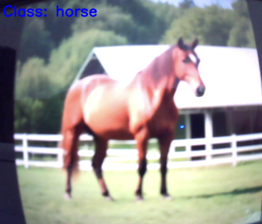
| import cv2 import numpy as np import tflite_runtime.interpreter as tflite # Set model path model_path = 'models/vgg16_20230801_040133.tflite' # Load tflite model interpreter = tflite.Interpreter(model_path=model_path) interpreter.allocate_tensors() # Get input and output details input_details = interpreter.get_input_details() output_details = interpreter.get_output_details() # CIFAR-10 class name class_names = ['airplane', 'automobile', 'bird', 'cat', 'deer', 'dog', 'frog', 'horse', 'ship', 'truck'] # Start input from USB camera cap = cv2.VideoCapture(0) while True: # Load frame from camera ret, frame = cap.read() if not ret: break #Resize image input_img = cv2.resize(frame, (32, 32)) # VGG16 model requires 32x32 images # OpenCV reads images in BGR format, so if your model is trained in RGB, convert it input_img = cv2.cvtColor(input_img, cv2.COLOR_BGR2RGB) # Normalization and type conversion input_img = input_img.astype(np.float32) / 255. input_img = np.expand_dims(input_img, axis=0) # Input images to the model and perform inference interpreter.set_tensor(input_details[0]['index'], input_img) interpreter.invoke() # Get inference results output_data = interpreter.get_tensor(output_details[0]['index']) print('output_data', output_data) class_id = np.argmax(output_data) # Draw inference results on an image cv2.putText(frame, 'Class: ' + class_names[class_id], (10, 50), cv2.FONT_HERSHEY_SIMPLEX, 1, (255, 0, 0), 2, cv2.LINE_AA) # Show Image cv2.imshow('Classification', frame) # Exit loop when q key is pressed if cv2.waitKey(1) & 0xFF == ord('q'): break # Close all windows cv2.destroyAllWindows() |
|---|
The image from the USB camera will be displayed, and the inference results (class names) will be displayed.
Afterword
We develop such AI applications and models, introduce and evaluate SoCs and accelerators for AI, and develop applications.
If you are interested, please Inquiry.
Inquiry
Related Product Information
An In-Depth Look at the Advantages of NXP's Automotive Microcontroller S32K1
NXP's S32K1 series of automotive microcontrollers incorporates the ARM Cortex-M0+ and M4F cores, achieving high processing power and low power consumption. We will thoroughly explain its appeal and features.
- NXP Semiconductors NV
- NEXT Mobility

Low-Power MCU with AI Accelerator for Edge AI
The MAX78000 series enables AI processing on low-power edge devices, enabling real-time processing of applications such as machine vision, audio, and facial recognition.
- Analog Devices, Inc.
- NEXT Mobility
- ICT and Industrial
- Smart Factories and Robotics
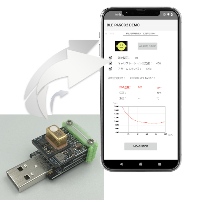
CO2センサーデモシステム
当社開発のCO2センサーデモシステムは、測定したCO2測定値をBLE経由で専用のAndroidアプリへ送信し、測定結果をグラフ表示可能です。
- Infineon Technologies AG
- ICT and Industrial
- Smart Factories and Robotics
The features and product lineup of the GMSL2 high-speed transmission technology for automotive applications
This article explains the features of Analog Devices' next-generation GMSL, GMSL2, which can handle video data from cameras with higher pixel counts.
- Analog Devices, Inc.
- NEXT Mobility
- ICT and Industrial

License control via CodeMeter soft files
CmActLicense, which allows license control using software files, effectively prevents illegal copying and use without the need for hardware.
- WIBU-SYSTEMS AG
- ICT and Industrial
- Smart Factories and Robotics
- Software
GMSL High-Speed Transmission Technology for Automotive Applications
This explains the high-speed transmission technology GMSL.
- Analog Devices, Inc.
- NEXT Mobility