Google Colaboratory上でCIFER10のモデルを学習および量⼦化し、エッジデバイス（RaspberryPi 3）で推論する

概要

この記事では、CIFAR-10データセットを使⽤してTensorFlowモデルを学習し、そのモデルを量⼦化し、Raspberry Pi 3での推論に使⽤する⽅法を説明します。

画像認識を活⽤するシーンが広がる中で、エッジデバイスによるリアルタイムでの認識処理が求められるユースケースが増加しています。

ネクスティエレクトロニクスではさまざまな画像認識・AIに関連するエッジデバイスを取り扱う中で画像認識・AIに関する取り組みを⾏っていますが、今回その取り組みの中の⼀つのサンプルとして、Google Colaboratoryを活⽤してモデルのトレーニングから量⼦化までを⾏い、最終的にRaspberry Pi 3で効率的な推論を実現する⼀連のプロセスを紹介します。

Google Colaboratoryの環境設定

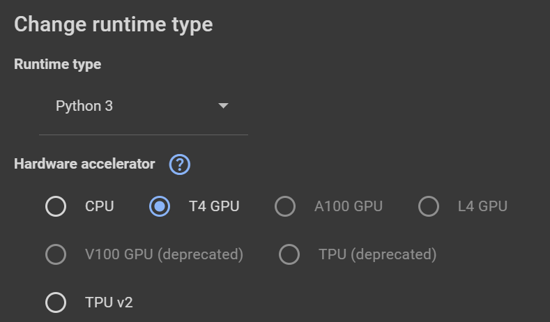
Menuの中からRuntimeChange runtime typeを選択し、T4 GPUを選択しました。

Google Driveのマウントとライブラリのインストール

まず、Google Driveをマウントし、必要なライブラリをインストールします。
（初回実⾏時にはGoogleドライブとの連携をするウィンドウが表⽰されるので、Googleアカウントでログインののち、接続をしてください。）

from google.colab import drive rive.mount('/content/gdrive') !pip install tensorflow==2.15.0

必要なライブラリのインポート

次に、必要なライブラリをインポートします。

import matplotlib.pyplot as plt
import numpy as np
import time
import datetime

from sklearn.metrics import accuracy_score, precision_score, recall_score,
f1_score

import keras
from keras.datasets import cifar10
from keras.applications import VGG16
from keras.layers import Dense, Flatten
from keras.models import Model
from keras.utils import to_categorical
from keras.optimizers import Adam
import tensorflow as tf
from tensorflow.keras import Input
from tensorflow.keras.layers import Conv2D, MaxPooling2D, Flatten, Dense

各モジュールのバージョン確認

print(f"Keras version: {keras.__version__}") print(f"TensorFlow version: {tf.__version__}") print(f"scikit-learn version: {sklearn.__version__}") print(f"matplotlib version: {matplotlib.__version__}") print(f"NumPy version: {np.__version__}")

Keras version: 2.15.0
TensorFlow version: 2.15.0
scikit-learn version: 1.2.2
matplotlib version: 3.7.1
NumPy version: 1.25.2

CIFAR－10 データセットの読み込みと前処理

CIFAR－10データセットを読み込み、前処理を⾏います。

# Load CIFAR10 data (train_images, train_labels), (test_images, test_labels) = cifar10.load_data() # Convert class vectors to binary class matrices. train_labels = to_categorical(train_labels, 10) test_labels = to_categorical(test_labels, 10) # Normalize pixel values to be between 0 and 1 train_images, test_images = train_images / 255.0, test_images / 255.0

モデルの選択と構築

VGG16を使⽤するか、カスタムモデルを使⽤するかを選択します。

この例ではあらかじめ⽤意されているVGG16モデルを使⽤しています。

use_vgg16 = True # This is the flag. If it is True, VGG16 is used. Otherwise,
your custom model is used.
model_name = ""

# 現在の⽇時を取得
now = datetime.datetime.now()

if use_vgg16:
# VGG16 Model
model_name = "vgg_16" + now.strftime("%Y%m%d_%H%M%S")

baseModel = VGG16(weights="imagenet", include_top=False, input_shape=(32,32, 3))
headModel = baseModel.output
headModel = Flatten(name="flatten")(headModel)
headModel = Dense(512, activation="relu")(headModel)
headModel = Dense(10, activation="softmax")(headModel)
model = Model(inputs=baseModel.input, outputs=headModel)
model.compile(optimizer=Adam(), loss='categorical_crossentropy', metrics=
['accuracy'])
else:
# Custom Model
model_name = "custom_model" + now.strftime("%Y%m%d_%H%M%S")
input_tensor = Input(shape=(32, 32, 3))

# Here you can manually change the number of layers, filters, kernel sizes
etc.
x = Conv2D(64, (3, 3), padding='same', activation='relu')(input_tensor)
x = Conv2D(64, (3, 3), padding='same', activation='relu')(x)
x = MaxPooling2D((2, 2))(x)

x = Conv2D(128, (3, 3), padding='same', activation='relu')(x)
x = Conv2D(128, (3, 3), padding='same', activation='relu')(x)
x = MaxPooling2D((2, 2))(x)

x = Conv2D(256, (3, 3), padding='same', activation='relu')(x)
x = Conv2D(256, (3, 3), padding='same', activation='relu')(x)
x = MaxPooling2D((2, 2))(x)

x = Flatten(name="flatten")(x)
x = Dense(512, activation="relu")(x)
output_tensor = Dense(10, activation="softmax")(x)

# Create the model
model = Model(inputs=input_tensor, outputs=output_tensor)
model.summary()

_________________________________________________________________
Layer (type) Output Shape Param #
=================================================================
input_3 (InputLayer) [(None, 32, 32, 3)] 0

block1_conv1 (Conv2D) (None, 32, 32, 64) 1792

block1_conv2 (Conv2D) (None, 32, 32, 64) 36928

block1_pool (MaxPooling2D) (None, 16, 16, 64) 0

block2_conv1 (Conv2D) (None, 16, 16, 128) 73856

block2_conv2 (Conv2D) (None, 16, 16, 128) 147584

block2_pool (MaxPooling2D) (None, 8, 8, 128) 0

block3_conv1 (Conv2D) (None, 8, 8, 256) 295168

block3_conv2 (Conv2D) (None, 8, 8, 256) 590080

block3_conv3 (Conv2D) (None, 8, 8, 256) 590080

block3_pool (MaxPooling2D) (None, 4, 4, 256) 0

block4_conv1 (Conv2D) (None, 4, 4, 512) 1180160

block4_conv2 (Conv2D) (None, 4, 4, 512) 2359808

block4_conv3 (Conv2D) (None, 4, 4, 512) 2359808

block4_pool (MaxPooling2D) (None, 2, 2, 512) 0

block5_conv1 (Conv2D) (None, 2, 2, 512) 2359808

block5_conv2 (Conv2D) (None, 2, 2, 512) 2359808

block5_conv3 (Conv2D) (None, 2, 2, 512) 2359808

block5_pool (MaxPooling2D) (None, 1, 1, 512) 0

flatten (Flatten) (None, 512) 0

dense_4 (Dense) (None, 512) 262656

dense_5 (Dense) (None, 10) 5130
=================================================================
Total params: 14982474 (57.15 MB)
Trainable params: 14982474 (57.15 MB)
Non-trainable params: 0 (0.00 Byte)
_________________________________________________________________

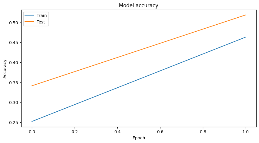
モデルの学習：2 Epochで実験

モデルをコンパイルし、学習を⾏います。
先に、Epochを2にして、あまり精度が⾼くないと思われる条件で学習を試します。

# Training epochs=2 model.compile(optimizer=Adam(), loss='categorical_crossentropy', metrics= ['accuracy']) history = model.fit(train_images, train_labels, batch_size=64, epochs=epochs, validation_data=(test_images, test_labels))

学習ログ抜粋

Epoch 1/2 782/782 [==============================]- 42s 41ms/step - loss: 1.8300 - accuracy: 0.2521 - val_loss: 1.6348 - val_accuracy: 0.3413 Epoch 2/2 782/782 [==============================] - 29s 38ms/step - loss: 1.3756 - accuracy: 0.4630 - val_loss: 1.3297 - val_accuracy: 0.5185

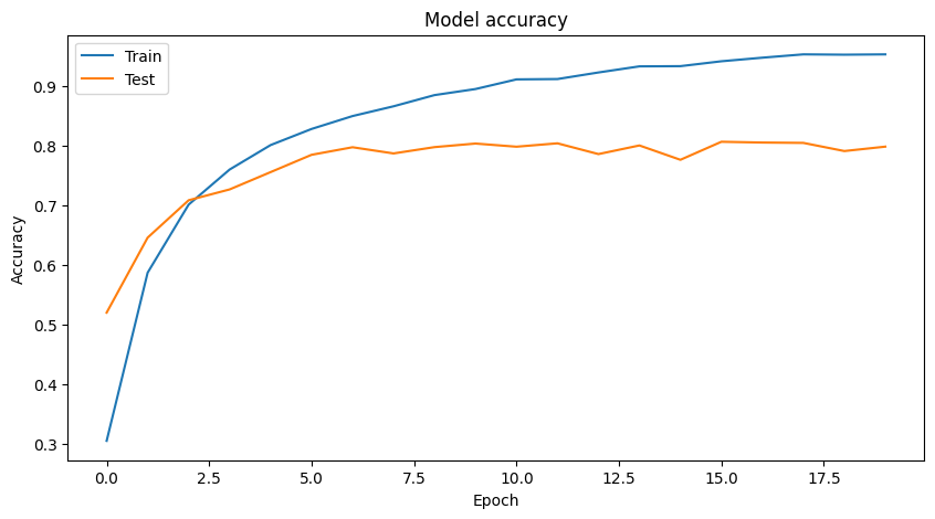
トレーニング結果の可視化

# Visualize Training Graph
# Plotting the accuracy
plt.figure(figsize=(10,5))
plt.plot(history.history['accuracy'])
plt.plot(history.history['val_accuracy'])
plt.title('Model accuracy')
plt.ylabel('Accuracy')
plt.xlabel('Epoch')
plt.legend(['Train', 'Test'], loc='upper left')
plt.show()

# Plotting the loss
plt.figure(figsize=(10,5))
plt.plot(history.history['loss'])
plt.plot(history.history['val_loss'])
plt.title('Model loss')
plt.ylabel('Loss')
plt.xlabel('Epoch')
plt.legend(['Train', 'Test'], loc='upper left')
plt.show()

モデルの評価と予測

# Predictions
class_names = ['airplane', 'automobile', 'bird', 'cat', 'deer', 'dog', 'frog',
'horse', 'ship', 'truck']

# Start time record
start_time = time.time()
# Predictions
predictions = model.predict(test_images)
# End time record
end_time = time.time()

# Convert predictions and test labels to 1D arrays
test_predictions = np.argmax(predictions, axis=1) # <-- Here we should use
'predictions'
test_labels_1d = np.argmax(test_labels, axis=1)

# Calculate accuracy
accuracy = accuracy_score(test_labels_1d, test_predictions)

# Calculate precision
precision = precision_score(test_labels_1d, test_predictions,
average='weighted')

# Calculate recall
recall = recall_score(test_labels_1d, test_predictions, average='weighted')

# Calculate F1 score
f1 = f1_score(test_labels_1d, test_predictions, average='weighted')

# Count the number of correct predictions
correct_predictions = np.sum(np.argmax(test_labels, axis=1) ==
np.argmax(predictions, axis=1))

# Calculate total inference time
total_inference_time = end_time - start_time

# Calculate inference time per image
inference_time_per_image = total_inference_time / test_images.shape[0]

# Calculate frames per second (fps)
fps = 1 / inference_time_per_image

# Calculate accuracy
test_accuracy = correct_predictions / test_images.shape[0]

# Get the number of model parameters
num_params = model.count_params()

print("\033[92m")
print("---Tensorflow")
print(f"Total inference time: {total_inference_time:.2f} seconds")
print(f"Inference time per image: {inference_time_per_image:.6f} seconds")
print(f"Inference speed: {fps:.2f} frames per second")
print(f"Test accuracy: {test_accuracy * 100:.2f}%")
print(f"Correct predictions: {correct_predictions}/{test_images.shape[0]}")
print(f"Accuracy: {accuracy}")
print(f"Precision: {precision}")
print(f"Recall: {recall}")
print(f"F1 Score: {f1}")
print(f"Number of parameters: {num_params}")
print(f"\033[0m")

---Tensorflow

Total inference time: 3.62 seconds
Inference time per image: 0.000362 seconds
Inference speed: 2762.24 frames per second
Test accuracy: 51.85%
Correct predictions: 5185/10000
Accuracy: 0.5185
Precision: 0.5460565026512546
Recall: 0.5185
F1 Score: 0.5121520088704362
Number of parameters: 14982474

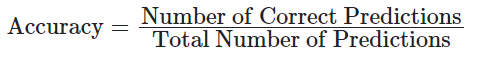
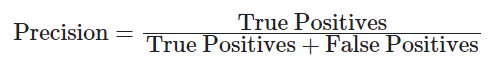
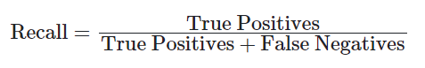
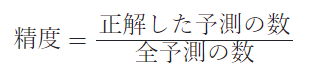
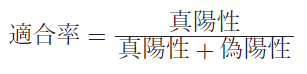
モデルの評価指標：英語版

以下の数式は、評価指標の計算⽅法を⽰しています。

精度（Accuracy）

Accuracy = Number of Correct Predictions / Total Number of Predictions

適合率（Precision）

Precision = True Positives / (True Positives + False Positives)

再現率（Recall）

Recall = True Positives / (True Positives + False Negatives)

F1スコア（F1 Score）

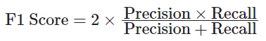
F1 Score = 2 × ((Precision × Recall) / (Precision + Recall))

モデルの評価指標：⽇本語版

以下の数式は、評価指標の計算⽅法を⽰しています。

精度（Accuracy）

適合率（Precision）

再現率（Recall）

F1スコア（F1 Score）

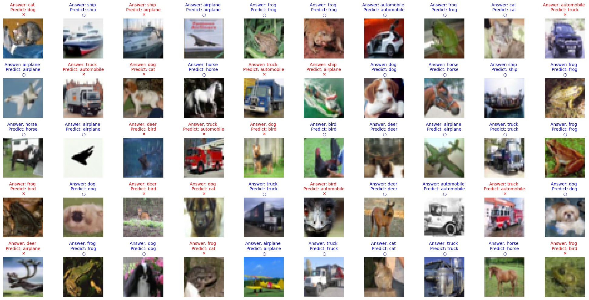
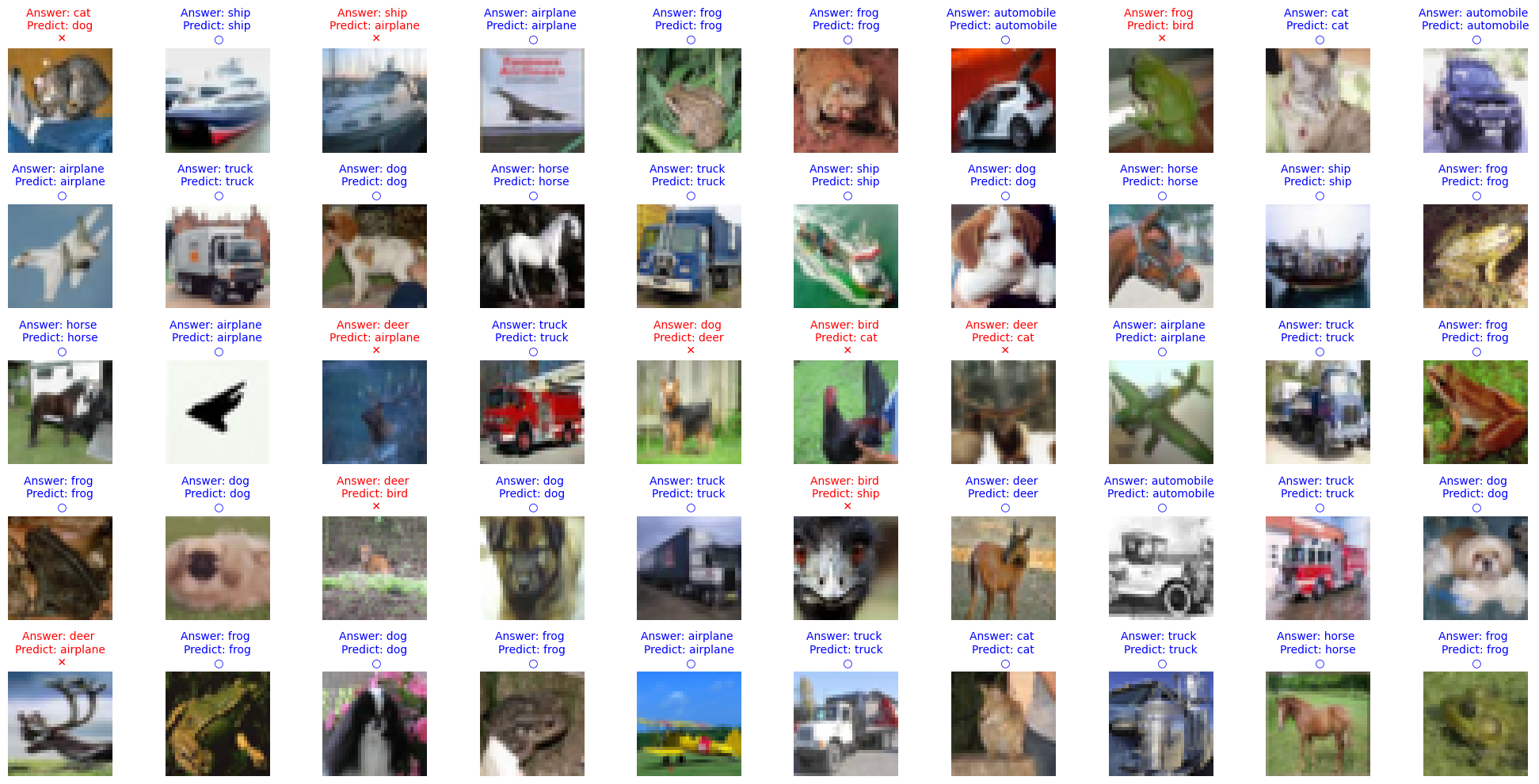
予測結果の可視化

正確な正解の数は上記のCorrect predictions: 5185/10000ですが、画像形式でも少し確認をしてみます。

テストデータからランダムに画像を表⽰し、正解と予測を⽐較します。

num_rows = 5
num_cols = 10
num_images = num_rows*num_cols

fig, axes = plt.subplots(num_rows, num_cols, figsize=(20, 2 * num_rows)) #
Adjust the figure size
axes = axes.ravel()

for i in np.arange(0, num_images):
axes[i].imshow(test_images[i])
if np.argmax(test_labels[i]) == np.argmax(predictions[i]):
axes[i].set_title("Answer: %s \nPredict: %s\n \u25CB" %
(class_names[np.argmax(test_labels[i])],

class_names[np.argmax(predictions[i])]), fontsize=10, color='blue')
else:
axes[i].set_title("Answer: %s \nPredict: %s\n \u2715" %
(class_names[np.argmax(test_labels[i])],

class_names[np.argmax(predictions[i])]), fontsize=10, color='red')
axes[i].axis('off')

plt.tight_layout() # Apply tight_layout

モデルの学習：20 Epochで実験

# Training epochs=20 model.compile(optimizer=Adam(), loss='categorical_crossentropy', metrics= ['accuracy']) history = model.fit(train_images, train_labels, batch_size=64, epochs=epochs, validation_data=(test_images, test_labels))

学習ログ抜粋

Epoch 1/20
782/782 [==============================] - 49s 51ms/step - loss: 1.7404 -
accuracy: 0.3044 - val_loss: 1.2784 - val_accuracy: 0.5199
Epoch 2/20
782/782 [==============================] - 33s 42ms/step - loss: 1.1353 -
accuracy: 0.5870 - val_loss: 1.0319 - val_accuracy: 0.6459
Epoch 3/20
782/782 [==============================] - 34s 44ms/step - loss: 0.8738 -
accuracy: 0.7014 - val_loss: 0.8739 - val_accuracy: 0.7087
Epoch 4/20
782/782 [==============================] - 38s 49ms/step - loss: 0.7150 -
accuracy: 0.7603 - val_loss: 0.7924 - val_accuracy: 0.7269
Epoch 5/20
782/782 [==============================] - 31s 40ms/step - loss: 0.6050 -
accuracy: 0.8014 - val_loss: 0.8037 - val_accuracy: 0.7560
Epoch 6/20
782/782 [==============================] - 31s 40ms/step - loss: 0.5321 -
accuracy: 0.8285 - val_loss: 0.6816 - val_accuracy: 0.7851
Epoch 7/20
782/782 [==============================] - 31s 40ms/step - loss: 0.4607 -
accuracy: 0.8502 - val_loss: 0.6683 - val_accuracy: 0.7978
Epoch 8/20
782/782 [==============================] - 32s 41ms/step - loss: 0.4130 -
accuracy: 0.8666 - val_loss: 0.6847 - val_accuracy: 0.7874
Epoch 9/20
782/782 [==============================] - 32s 41ms/step - loss: 0.3603 -
accuracy: 0.8854 - val_loss: 0.6863 - val_accuracy: 0.7980
Epoch 10/20
782/782 [==============================] - 32s 41ms/step - loss: 0.3283 -
accuracy: 0.8956 - val_loss: 0.7302 - val_accuracy: 0.8040
Epoch 11/20
782/782 [==============================] - 31s 40ms/step - loss: 0.2775 -
accuracy: 0.9118 - val_loss: 0.7026 - val_accuracy: 0.7987
Epoch 12/20
782/782 [==============================] - 31s 40ms/step - loss: 0.2710 -
accuracy: 0.9124 - val_loss: 0.7211 - val_accuracy: 0.8044
Epoch 13/20
782/782 [==============================] - 31s 40ms/step - loss: 0.2417 -
accuracy: 0.9235 - val_loss: 0.7624 - val_accuracy: 0.7863
Epoch 14/20
782/782 [==============================] - 32s 41ms/step - loss: 0.2163 -
accuracy: 0.9337 - val_loss: 0.8034 - val_accuracy: 0.8008
Epoch 15/20
782/782 [==============================] - 31s 40ms/step - loss: 0.2113 -
accuracy: 0.9341 - val_loss: 0.8858 - val_accuracy: 0.7767
Epoch 16/20
782/782 [==============================] - 31s 39ms/step - loss: 0.1905 -
accuracy: 0.9423 - val_loss: 0.7814 - val_accuracy: 0.8070
Epoch 17/20
782/782 [==============================] - 31s 40ms/step - loss: 0.1669 -
accuracy: 0.9483 - val_loss: 0.8559 - val_accuracy: 0.8057
Epoch 18/20
782/782 [==============================] - 31s 40ms/step - loss: 0.1532 -
accuracy: 0.9539 - val_loss: 0.8492 - val_accuracy: 0.8051
Epoch 19/20
782/782 [==============================] - 31s 40ms/step - loss: 0.1540 -
accuracy: 0.9534 - val_loss: 0.8842 - val_accuracy: 0.7914
Epoch 20/20
782/782 [==============================] - 32s 41ms/step - loss: 0.1515 -
accuracy: 0.9539 - val_loss: 0.9053 - val_accuracy: 0.7988

トレーニング結果の可視化

学習過程の正確性と損失をプロットします。

# Visualize Training Graph
# Plotting the accuracy
plt.figure(figsize=(10,5))
plt.plot(history.history['accuracy'])
plt.plot(history.history['val_accuracy'])
plt.title('Model accuracy')
plt.ylabel('Accuracy')
plt.xlabel('Epoch')
plt.legend(['Train', 'Test'], loc='upper left')
plt.show()
# Plotting the loss
plt.figure(figsize=(10,5))
plt.plot(history.history['loss'])
plt.plot(history.history['val_loss'])
plt.title('Model loss')
plt.ylabel('Loss')
plt.xlabel('Epoch')
plt.legend(['Train', 'Test'], loc='upper left')
plt.show()

モデルの評価と予測

テストデータを⽤いてモデルの性能を評価し、予測結果を出⼒します。

# Predictions
class_names = ['airplane', 'automobile', 'bird', 'cat', 'deer', 'dog', 'frog',
'horse', 'ship', 'truck']

# Start time record
start_time = time.time()
# Predictions
predictions = model.predict(test_images)
# End time record
end_time = time.time()

# Convert predictions and test labels to 1D arrays
test_predictions = np.argmax(predictions, axis=1)
test_labels_1d = np.argmax(test_labels, axis=1)

# Calculate accuracy
accuracy = accuracy_score(test_labels_1d, test_predictions)

# Calculate precision
precision = precision_score(test_labels_1d, test_predictions,
average='weighted')

# Calculate recall
recall = recall_score(test_labels_1d, test_predictions, average='weighted')

# Calculate F1 score
f1 = f1_score(test_labels_1d, test_predictions, average='weighted')

# Count the number of correct predictions
correct_predictions = np.sum(np.argmax(test_labels, axis=1) ==
np.argmax(predictions, axis=1))

# Calculate total inference time
total_inference_time = end_time - start_time

# Calculate inference time per image
inference_time_per_image = total_inference_time / test_images.shape[0]

# Calculate frames per second (fps)
fps = 1 / inference_time_per_image

# Calculate accuracy
test_accuracy = correct_predictions / test_images.shape[0]

# Get the number of model parameters
num_params = model.count_params()

print("\033[92m")
print("---Tensorflow")
print(f"Total inference time: {total_inference_time:.2f} seconds")
print(f"Inference time per image: {inference_time_per_image:.6f} seconds")
print(f"Inference speed: {fps:.2f} frames per second")
print(f"Test accuracy: {test_accuracy * 100:.2f}%")
print(f"Correct predictions: {correct_predictions}/{test_images.shape[0]}")
print(f"Accuracy: {accuracy}")
print(f"Precision: {precision}")
print(f"Recall: {recall}")
print(f"F1 Score: {f1}")
print(f"Number of parameters: {num_params}")
print("\033[0m")

---Tensorflow

Total inference time: 3.44 seconds
Inference time per image: 0.000344 seconds
Inference speed: 2910.39 frames per second
Test accuracy: 79.88%
Correct predictions: 7988/10000
Accuracy: 0.7988
Precision: 0.8079718674357317
Recall: 0.7988
F1 Score: 0.8000619454577802
Number of parameters: 14982474

予測結果の可視化

テストデータからランダムに画像を表⽰し、正解と予測を⽐較します。

num_rows = 5
num_cols = 10
num_images = num_rows*num_cols

fig, axes = plt.subplots(num_rows, num_cols, figsize=(20, 2 * num_rows)) #
Adjust the figure size
axes = axes.ravel()

for i in np.arange(0, num_images):
axes[i].imshow(test_images[i])
if np.argmax(test_labels[i]) == np.argmax(predictions[i]):
axes[i].set_title("Answer: %s \nPredict: %s\n \u25CB" %
(class_names[np.argmax(test_labels[i])],

class_names[np.argmax(predictions[i])]), fontsize=10, color='blue')
else:
axes[i].set_title("Answer: %s \nPredict: %s\n \u2715" %
(class_names[np.argmax(test_labels[i])],
class_names[np.argmax(predictions[i])]), fontsize=10, color='red')
axes[i].axis('off')
plt.tight_layout() # Apply tight_layout

Epoch2とEpoch20の⽐較

指標	Epoch2	Epoch20
精度（Accuracy）	0.5185（51.85％）	0.7988（79.88％）
Precision（適合率）	0.5461	0.8080
Recall（再現率）	0.5185	0.7988
F1スコア	0.5122	0.8001

Accuracy

Epoch2の精度は51.85％であり、これはモデルがランダムに予測しているわけではないものの、ほぼ半分の精度であることを⽰しています。
Epoch20では79.88％の精度に向上しており、モデルがより正確に分類できるようになったことがわかります。

Precision

Precisionは正しく分類された正例の割合を⽰します。
Epoch2では0.5461でしたが、Epoch20では0.8080に向上しています。
これはモデルが正例をより正確に予測できるようになったことを⽰しています。

Recall

Recallは全体の正例の中で正しく分類された割合を⽰します。
Epoch2では0.5185でしたが、Epoch20では0.7988に向上しています。
これはモデルが多くの正例を⾒逃さずに予測できるようになったことを⽰しています。

F1スコア

F1スコアはPrecisionとRecallの調和平均であり、バランスの取れた評価指標です。
Epoch2では0.5122でしたが、Epoch20では0.8001に向上しています。
これはモデルが全体としてよりバランスの取れたパフォーマンスを発揮していることを⽰しています。

総合評価

Epoch2とEpoch20を⽐較すると、Epoch20のモデルが明らかに優れていることがわかります。学習を続けることで、モデルの精度、推論速度、Precision、Recall、およびF1スコアの全てが向上しています。
これは、モデルがより多くのデータを学習し、パラメータの最適化が進んだためと考えられます。

その他補⾜

モデルの学習過程

初期のエポックではモデルがまだ最適な重みを⾒つける途中であるため、精度や他の指標が低い傾向にあります。Epoch数を増やすことで、モデルはデータの特徴をよりよく学習し、パラメータの調整が進み、性能が向上します。

オーバーフィッティングの懸念

エポック数が増えると、学習データに対する過剰適合（オーバーフィッティング）のリスクが⾼まります。現時点では、エポック20の結果から、オーバーフィッティングの兆候は⾒られませんが、学習の継続には検証データセットでの評価が重要です。

ハイパーパラメータチューニング

学習率やバッチサイズなどのハイパーパラメータのチューニングがモデルの性能に影響を与える可能性があります。適切なハイパーパラメータを⾒つけることが重要です。

総じて、Epoch数を増やすことでモデルの精度が⼤幅に向上していることが確認でき、学習過程が順調に進んでいることが⽰されています。

Kerasモデルの保存

このブロックは、訓練済みのKerasモデルをHDF5形式（.h5）で保存します。

model_name変数を使⽤してモデルファイルのフルパスを定義し、model.saveを使⽤してモデルを保存します。

full_model_name_h5 = "/content/gdrive/MyDrive/Colab Notebooks/{}.h5".format(model_name) model.save(full_model_name_h5)

モデルをTensorFlow Liteに変換

このブロックは、保存されたKerasモデルをTensorFlow Lite形式に変換します。

まず、tf.keras.models.load_modelを使⽤してモデルをロードします。

次に、TFLiteConverterオブジェクトを作成し、量⼦化を使⽤してモデルを変換するように設定します（converter.optimizations = [tf.lite.Optimize.DEFAULT]）。

最後に、モデルを変換し、変換されたデータをtflite_model変数に格納します。

import tensorflow as tf

# Load the model
model = tf.keras.models.load_model(full_model_name_h5)

# Convert the model to the TensorFlow Lite format with quantization
converter = tf.lite.TFLiteConverter.from_keras_model(model)
# Conveert float32 to int8
converter.optimizations = [tf.lite.Optimize.DEFAULT]
tflite_model = converter.convert()

# Save the model to disk
full_model_name_tflite = "/content/gdrive/MyDrive/Colab
Notebooks/{}.tflite".format(model_name)

open(full_model_name_tflite, "wb").write(tflite_model)

TensorFlow Liteモデルでの読み込みと推論の実⾏

変換されたTensorFlow Liteモデルをロードし、単⼀のテスト画像に対して推論を実⾏します。

1.TFLiteInterpreterオブジェクトを作成し、モデルパスを指定してテンソルにメモリを割り当てます。
2.次に、⼊⼒と出⼒テンソルの詳細を取得します。テスト画像を再整形してfloat32形式に変換することで、⼊⼒データを準備します。
3.準備されたデータが指すように⼊⼒テンソルを設定し、interpreter.invokeを使⽤して推論を実⾏します。
4.最後に、出⼒データを取得し、出⼒の最⼤値に基づいて予測クラスを取得します。

# Load TFLite model and allocate tensors
interpreter = tf.lite.Interpreter(model_path=full_model_name_tflite)
interpreter.allocate_tensors()

# Get input and output tensors
input_details = interpreter.get_input_details()
output_details = interpreter.get_output_details()

# Prepare the input data
input_shape = input_details[0]['shape']
input_data = np.expand_dims(test_images[i], axis=0).astype("float32") #
Assuming you are checking for `i`th image

# Set the tensor to point to the input data to be inferred
interpreter.set_tensor(input_details[0]['index'], input_data)

# Run the inference
interpreter.invoke()

# Get the output from the inference
output_data = interpreter.get_tensor(output_details[0]['index'])

# Get the output class
output_class = np.argmax(output_data)

TensorFlow Liteモデルのパフォーマンス評価

TensorFlow Liteモデルのパフォーマンスをテストデータセット全体で評価します。

1.評価指標を計算するために必要なライブラリをインポートします。モデルから⼊⼒形状を取得することで、⼊⼒データを準備します。
2.すべてのテスト画像に対する予測を格納するリストpredictionsを作成します。時間を記録し始め、すべてのテスト画像を反復処理します。
3.ループ内で、各画像の⼊⼒データを準備し、⼊⼒テンソルを設定し、推論を実⾏し、出⼒を取得し、予測をpredictionsリストに追加します。
4.すべての画像を反復処理した後、時間を記録します。予測とテストラベルを1D配列に変換して、⽐較を容易にします。
5.sklearn.metricsの関数を使⽤して、精度、精度、再現率、F1スコアなどのさまざまな評価指標を計算します。
6.最後に、合計推論時間、画像あたりの推論時間、フレームレート（FPS）を計算し、モデルのパラメータ数とともに結果を出⼒します。

# Import necessary libraries
import time
from sklearn.metrics import accuracy_score, precision_score, recall_score,
f1_score

# Prepare the input data
input_shape = input_details[0]['shape']

# Placeholder for predictions
predictions = []

# Start time record
start_time = time.time()
# Run the inference for each test image
for i in range(len(test_images)):
input_data = np.expand_dims(test_images[i], axis=0).astype("float32")
interpreter.set_tensor(input_details[0]['index'], input_data)
interpreter.invoke()
output_data = interpreter.get_tensor(output_details[0]['index'])
predictions.append(output_data)

# End time record
end_time = time.time()

predictions = np.array(predictions).squeeze()

# Convert predictions and test labels to 1D arrays
test_predictions = np.argmax(predictions, axis=1)
test_labels_1d = np.argmax(test_labels, axis=1)

# Calculate accuracy
accuracy = accuracy_score(test_labels_1d, test_predictions)

# Calculate precision
precision = precision_score(test_labels_1d, test_predictions,
average='weighted')

# Calculate recall
recall = recall_score(test_labels_1d, test_predictions, average='weighted')

# Calculate F1 score
f1 = f1_score(test_labels_1d, test_predictions, average='weighted')

# Count the number of correct predictions
correct_predictions = np.sum(test_labels_1d == test_predictions)

# Calculate accuracy
test_accuracy = correct_predictions / test_images.shape[0]

print("\033[92m")
print("---Tensorflow Lite")
print(f"Test accuracy: {test_accuracy * 100:.2f}%")
print(f"Correct predictions: {correct_predictions}/{test_images.shape[0]}")
print(f"Accuracy: {accuracy}")
print(f"Precision: {precision}")
print(f"Recall: {recall}")
print(f"F1 Score: {f1}")
print(f"Number of parameters: {num_params}")
print(f"\033[0m")

---Tensorflow Lite

Test accuracy: 79.78%
Correct predictions: 7978/10000
Accuracy: 0.7978
Precision: 0.8069027338990966
Recall: 0.7978
F1 Score: 0.7990733190498165
Number of parameters: 14982474

予測の可視化

このブロックは、テスト画像とその予測ラベルと真のラベルを可視化します。

1.画像を表⽰する⾏と列の数と定義し、Matplotlibを使⽤してサブプロットを含む図を作成します。
2.すべてのテスト画像を反復処理し、imshowを使⽤して表⽰します。予測クラスが真のクラスと⼀致するかどうかを確認します。
3.⼀致する場合、⻘⾊の丸（○）でタイトルを設定し、正しい予測であることを⽰します。
4.⼀致しない場合は、⾚い×（×）でタイトルを設定し、誤った予測であることを⽰します。各サブプロットの軸ラベルをオフにし、より良い整理のためにタイトレイアウトを適⽤します。

モデルサイズの⽐較

学習済みモデルのサイズを表⽰し、H5形式とTFLite形式の圧縮率を計算します。

import os

# Model file paths
h5_model_file = full_model_name_h5
tflite_model_file = full_model_name_tflite

# Get file sizes
h5_model_size = os.path.getsize(h5_model_file) / 1024 / 1024 # Size in
megabytes
tflite_model_size = os.path.getsize(tflite_model_file) / 1024 / 1024 # Size in
megabytes

print(f"Size of H5 model: {h5_model_size:.2f} MB")
print(f"Size of TFLite model: {tflite_model_size:.2f} MB")
print(f"Compression rate: {h5_model_size / tflite_model_size:.2f} times")

---Tensorflow Lite

Size of H5 model: 171.59 MB
Size of TFLite model: 14.36 MB
Compression rate: 11.95 times

量⼦化前後のモデル性能とサイズの⽐較

	量⼦化前	量⼦化後
Test accuracy	79.88%	79.78%
Correct predictions	7988/10000	7978/10000
Accuracy	0.7988	0.7978
Precision	0.8079718674357317	0.8069027338990966
Recall	0.7988	0.7978
F1 Score	0.8000619454577802	0.7990733190498165
Number of parameters	14,982,474	14,982,474
Model size	171.59 MB	14.36 MB
Compression rate	-	11.95 (約12倍)

Test accuracy（テスト精度）

量⼦化前: 79.88％
量⼦化後: 79.78％

テスト精度に関してはわずかな低下が⾒られますが、ほぼ同等のパフォーマンスを維持しています。これは、量⼦化がモデルの精度に⼤きな影響を与えないことを⽰しています。

Correct predictions（正しい予測数）

量⼦化前: 7988/10000
量⼦化後: 7978/10000

正しく予測された数もほぼ同じであり、量⼦化がモデルの性能に与える影響はごくわずかであることがわかります。

Accuracy（精度）

量⼦化前: 0.7988
量⼦化後: 0.7978

精度はわずかに低下していますが、依然として⾼い⽔準を維持しています。
これにより、量⼦化後のモデルが実⽤上問題のないレベルの精度を持っていることが確認できます。

Precision（適合率）

量⼦化前: 0.8079718674357317
量⼦化後: 0.8069027338990966

適合率もほぼ同等であり、量⼦化後のモデルが依然として⾼い精度を保っていることがわかります。
これは、量⼦化が誤検出を増やすことなく精度を維持していることを⽰しています。

Recall（再現率）

量⼦化前: 0.7988
量⼦化後: 0.7978

再現率もほぼ同じであり、量⼦化による影響はごくわずかです。
モデルは依然として多くの正例を正しく検出する能⼒を維持しています。

F1 Score（F1スコア）

量⼦化前: 0.8000619454577802
量⼦化後: 0.7990733190498165

F1スコアもわずかに低下していますが、依然として⾼い⽔準を維持しています。
これにより、量⼦化後のモデルがバランスの取れた性能を発揮していることがわかります。

Number of parameters（パラメータ数）

量⼦化前: 14,982,474
量⼦化後: 14,982,474

変化なし。

パラメータ数は量⼦化前後で変わりませんが、量⼦化により各パラメータの形式が変わっています。
これにより、メモリ使⽤量が削減され、モデルのサイズが圧縮されています。

まとめ

量⼦化前後のモデルを⽐較すると、量⼦化後のモデルは⼤幅に圧縮され、モデルサイズが⼤幅に減少している。
⼀⽅で、精度やその他の評価指標においてはほとんど変化がないことがわかる。
これは、量⼦化がメモリ使⽤量を削減し、ストレージや転送効率を改善しつつ、モデルのパフォーマンスをほぼ維持できる有効な⼿法であることを⽰している。
特に、リソースが限られた環境でのデプロイや運⽤において、量⼦化は⾮常に有⽤である。

補⾜

モデルの量⼦化には他にもいくつかオプションがある。

TensorFlow tf.lite.Optimize詳細ページへ

保存されたモデルについて

正常に動作した場合、GdriveのColab Notebooksディレクトリ以下にxxx.h5、xxx.tfliteが保存される

これをダウンロードローカルPCにダウンロードします。
例: ./Desktop/models/vgg_16_20230714_021101.tflite

Raspberry Pi + USB Cameraでの推論動作

環境

デバイス: Raspberry Pi 3 Model B+
カメラ: USB Camera(解像度に関しては、推論コード内でリサイズ処理が⼊っているため特に指定なし)
IPアドレス:
ifconfigコマンドなどで、事前にRaspberry PiのIPアドレスを調べておく。
例: 169.254.112.21

データの転送

上記で作成した量⼦化後のモデルをRaspberry Piへ転送する
scp -r ./Desktop/models/vgg_16_20230714_021101.tflite
pi@169.254.112.216:/home/pi/vgg16/

推論

requirements.txt

flatbuffers==20181003210633 numpy==1.25.1 opencv-python==4.5.1.48 pkg_resources==0.0.0 tflite==2.10.0 tflite-runtime==2.13.0

必要なモジュールのインストール

pip install -r requirements.txt

推論コード(tf_inference.py)

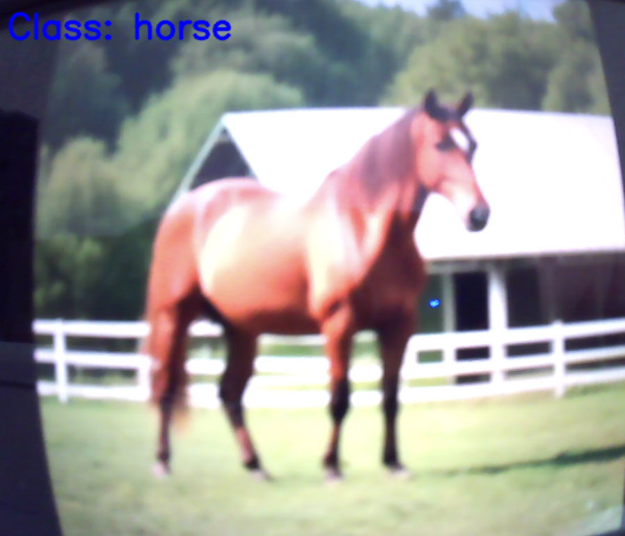
import cv2
import numpy as np
import tflite_runtime.interpreter as tflite

# Set model path
model_path = ‘models/vgg16_20230801_040133.tflite’

# Load tflite model
interpreter = tflite.Interpreter(model_path=model_path)
interpreter.allocate_tensors()

# Get input and output details
input_details = interpreter.get_input_details()
output_details = interpreter.get_output_details()

# CIFAR-10 class name
class_names = [‘airplane’, ‘automobile’, ‘bird’, ‘cat’, ‘deer’, ‘dog’, ‘frog’,
‘horse’, ‘ship’, ‘truck’]

# Start input from USB camera
cap = cv2.VideoCapture(0)

while True:
# Load frame from camera
ret, frame = cap.read()
if not ret:
break
#Resize image

input_img = cv2.resize(frame, (32, 32)) # VGG16 model requires 32x32
images
# OpenCV reads images in BGR format, so if your model is trained in RGB,
convert it
input_img = cv2.cvtColor(input_img, cv2.COLOR_BGR2RGB)

# Normalization and type conversion
input_img = input_img.astype(np.float32) / 255.
input_img = np.expand_dims(input_img, axis=0)

# Input images to the model and perform inference
interpreter.set_tensor(input_details[0][‘index’], input_img)
interpreter.invoke()

# Get inference results
output_data = interpreter.get_tensor(output_details[0][‘index’])
print(‘output_data’, output_data)
class_id = np.argmax(output_data)

# Draw inference results on an image
cv2.putText(frame, ‘Class: ’ + class_names[class_id], (10, 50),
cv2.FONT_HERSHEY_SIMPLEX, 1, (255, 0, 0), 2, cv2.LINE_AA)

# Show Image
cv2.imshow(‘Classification’, frame)

# Exit loop when q key is pressed
if cv2.waitKey(1) & 0xFF == ord(‘q’):
break

# Close all windows
cv2.destroyAllWindows()

USBカメラの画像が表⽰され、推論結果（クラス名）が表⽰されます。

あとがき

弊社では、このようなAIアプリ／モデルの開発や、AI向けのSoC／アクセラレータのご紹介や、評価、アプリ開発などを⾏っております。

ご興味のある⽅はぜひお問い合わせください。

お問い合わせ

お問い合わせをする

概要

Google Colaboratoryの環境設定

Google Driveのマウントとライブラリのインストール

必要なライブラリのインポート

各モジュールのバージョン確認

CIFAR－10 データセットの読み込みと前処理

モデルの選択と構築

モデルの学習：2 Epochで実験

モデルの学習：20 Epochで実験

Epoch2とEpoch20の⽐較

Kerasモデルの保存

モデルをTensorFlow Liteに変換

TensorFlow Liteモデルでの読み込みと推論の実⾏

TensorFlow Liteモデルのパフォーマンス評価

予測の可視化

モデルサイズの⽐較

量⼦化前後のモデル性能とサイズの⽐較

保存されたモデルについて

Raspberry Pi + USB Cameraでの推論動作

あとがき

お問い合わせ

関連製品情報

概要

Google Colaboratoryの環境設定

Google Driveのマウントとライブラリのインストール

必要なライブラリのインポート

各モジュールのバージョン確認

CIFAR－10 データセットの読み込みと前処理

モデルの選択と構築

モデルの学習：2 Epochで実験

モデルの学習：20 Epochで実験

Epoch2とEpoch20の⽐較

Kerasモデルの保存

モデルをTensorFlow Liteに変換

TensorFlow Liteモデルでの読み込みと推論の実⾏

TensorFlow Liteモデルのパフォーマンス評価

予測の可視化

モデルサイズの⽐較

量⼦化前後のモデル性能とサイズの⽐較

保存されたモデルについて

Raspberry Pi + USB Cameraでの推論動作

あとがき

お問い合わせ

関連製品情報